Supply Chain Web App
Building a simple supply chain web app
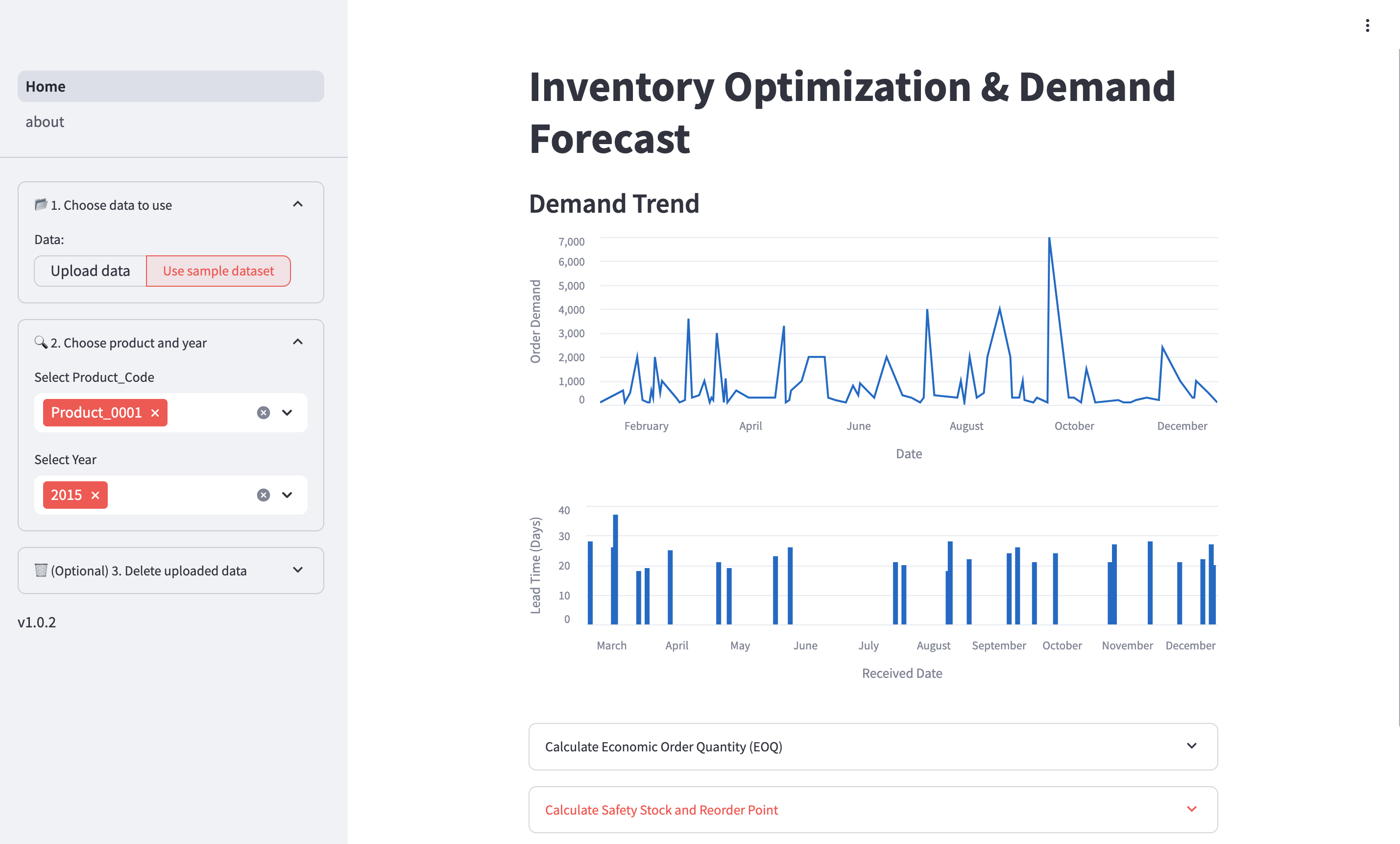
I wanted to learn more about data science in supply chain, particularly in inventory optimization and demand forecasting, so I decided to build a web app and deploy it on the cloud, with CI/CD setup. Here’s how I did it.
App
GitHub
Demo
Tech Stack
- Frontend: Streamlit
- Backend: Nginx
- Cloud: AWS EC2
- Tools: Darts
- CI/CD: GitHub Actions, Docker, Pytest, Streamlit AppTest
Architecture
Step 1: Preparing datasets
Firstly, I need the product demand and lead time datasets for simulating the inventory and predicting the demand. For the product demand, I utilized the Historical Product Demand dataset from Kaggle. This dataset consists of the daily product demand with their product code, warehouse, and product category.
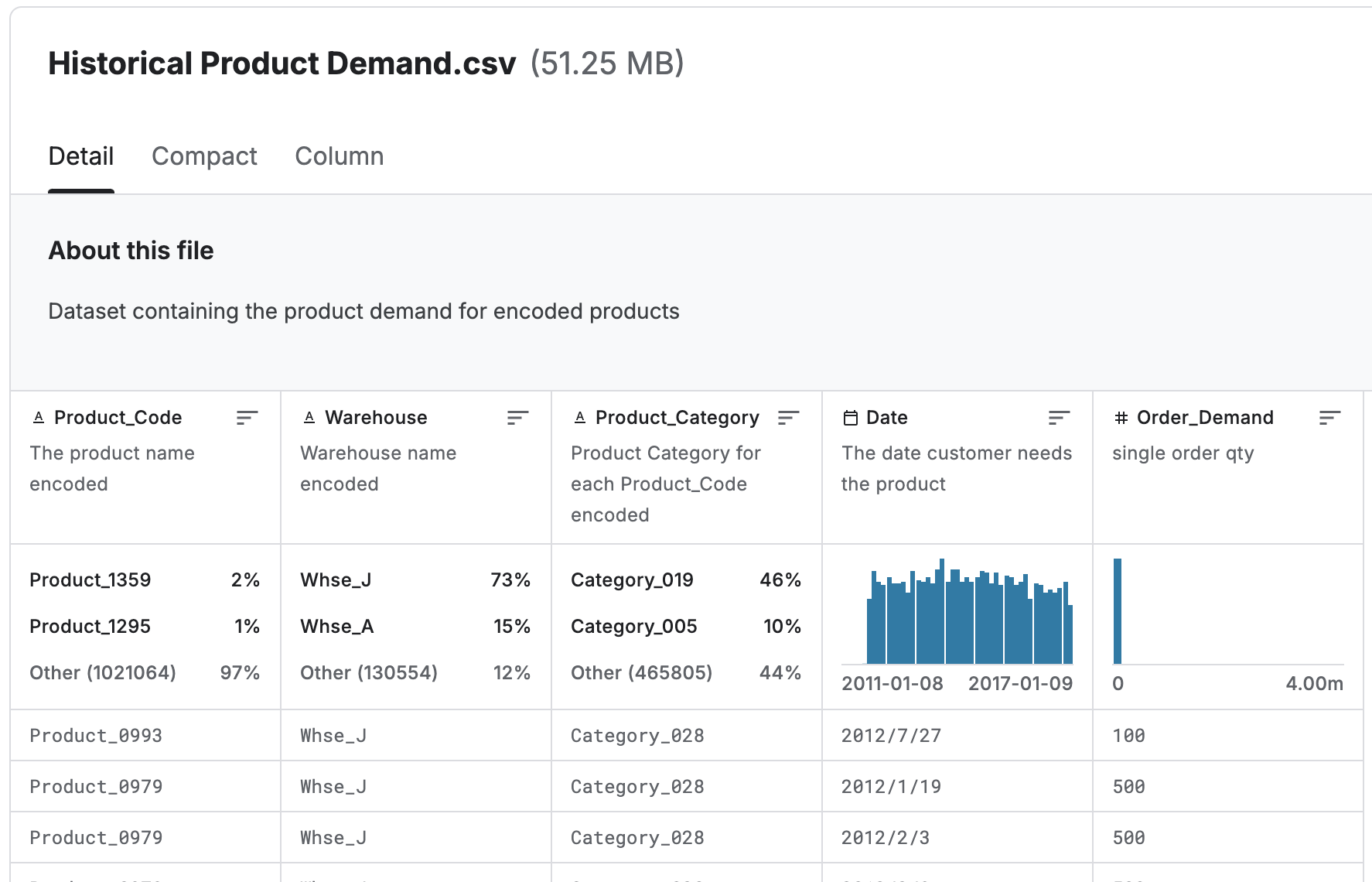
For the lead time data, I wrote a script to generate synthetic lead time dataset based on the product demand sample dataset.
Step 2: Developing the application
There are 5 main functionalities for this application:
- Visualizing demand trend and lead time distributions
- Calculating supply chain metrics
- Simulating inventory on actual demand
- Forecasting demand
- Uploading custom demand trend and lead time datasets
Visualizing demand trend and lead time distributions
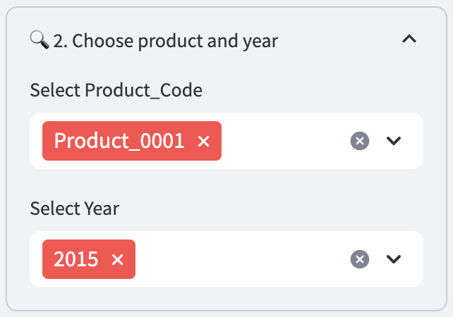
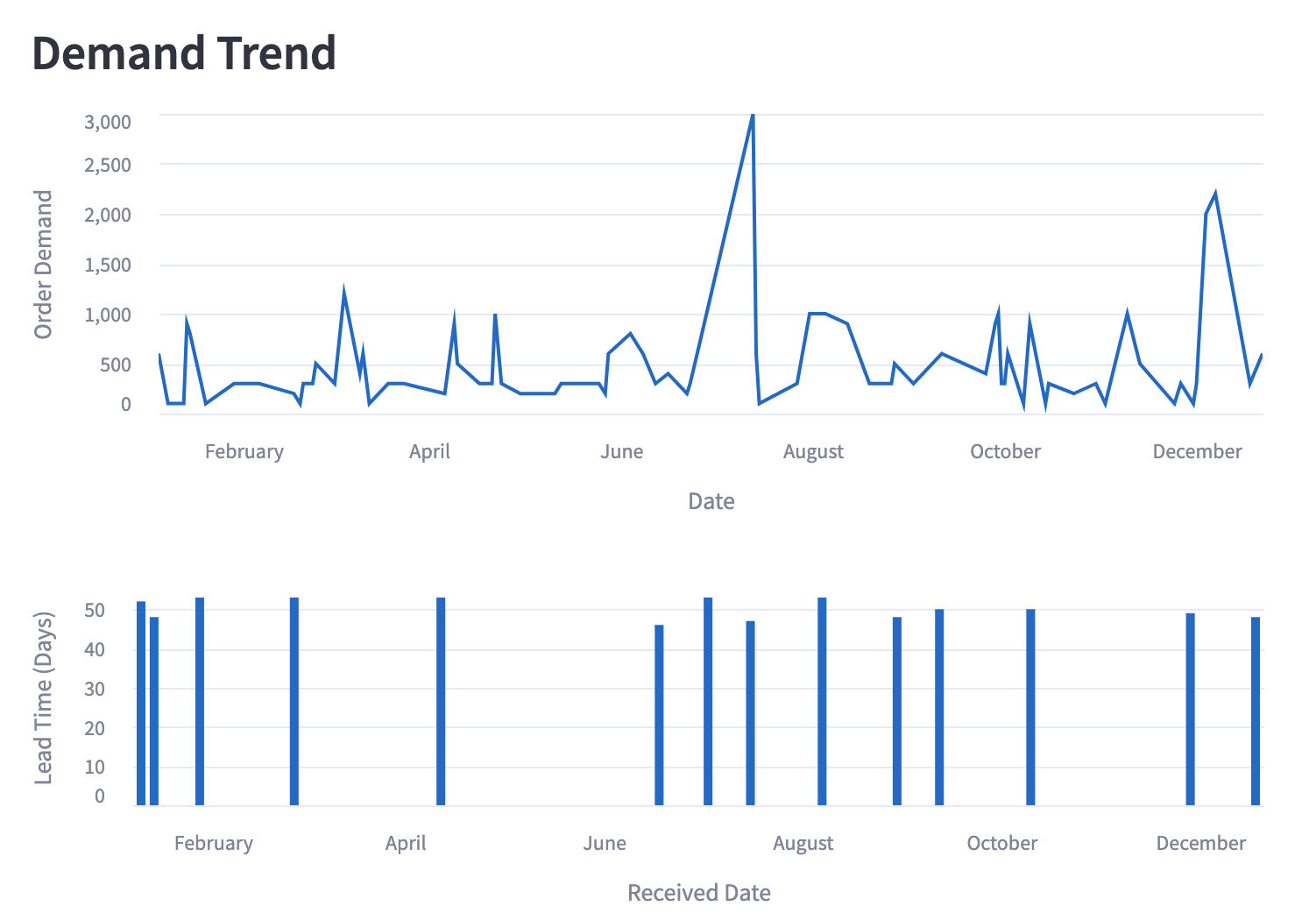
I started by developing the filters to allow user to choose the product and year. The year is based on the Date field in the product demand sample dataset.
After that, I developed the charts to plot the demand trend and lead time distributions.
Calculating supply chain metrics (inventory optimization)
After looking at the trend and distribution, now the user will have a good idea of what is happening. To enable users to perform inventory optimization, I then move on to implement functions to compute the supply chain metrics (economic order quantity, safety stock and reorder point). These functionalities will automatically calculate these metrics based on the product demand and lead time data after user selected the product code and year. They also allow user to adjust the inputs.
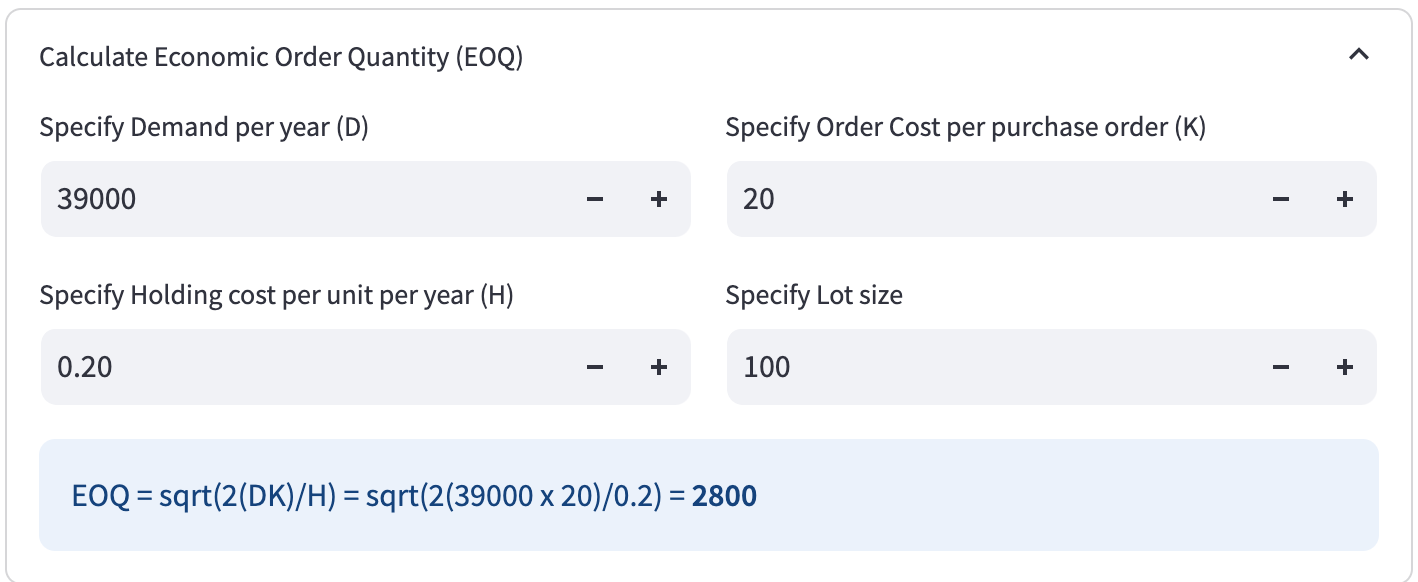
For the Economic Order Quantity, the default value for Demand per year is the total demand based on the product code and year that user selected. The default values for other inputs are arbitrary numbers. Note: EOQ is used here for demonstratice purposes. For the highly variable demand patterns shown in the dataset, dynamic probabilistic sizing would be more appropriate.
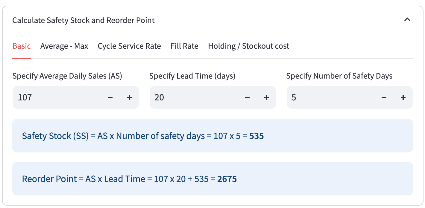
For the Safety Stock and Reorder Point, I referenced the Basic, Average - Max, Cycle Service Rate formulas from here (Credits to Edouard Thieuleux) and Fill Rate, Holding/Stockout Cost formulas from here. The default values for Average Daily Sales and Lead Time (days) are the average daily product demand, average lead time (days) based on the product code and year that user selected.
Simulating inventory on actual demand
With the supply chain metrics ready, I wanted to verify them through simulation. User need to select the year to simulate. Then, user need to specify the Safety Stock, Reorder Point, Order Quantity based on the values calculated previously. The default value for Average Lead Time (days) is the average lead time (days) based on the product code and year that user selected. Upon providing all the inputs, a line chart will appear to simulate the daily inventory quantity and product demand in the year.
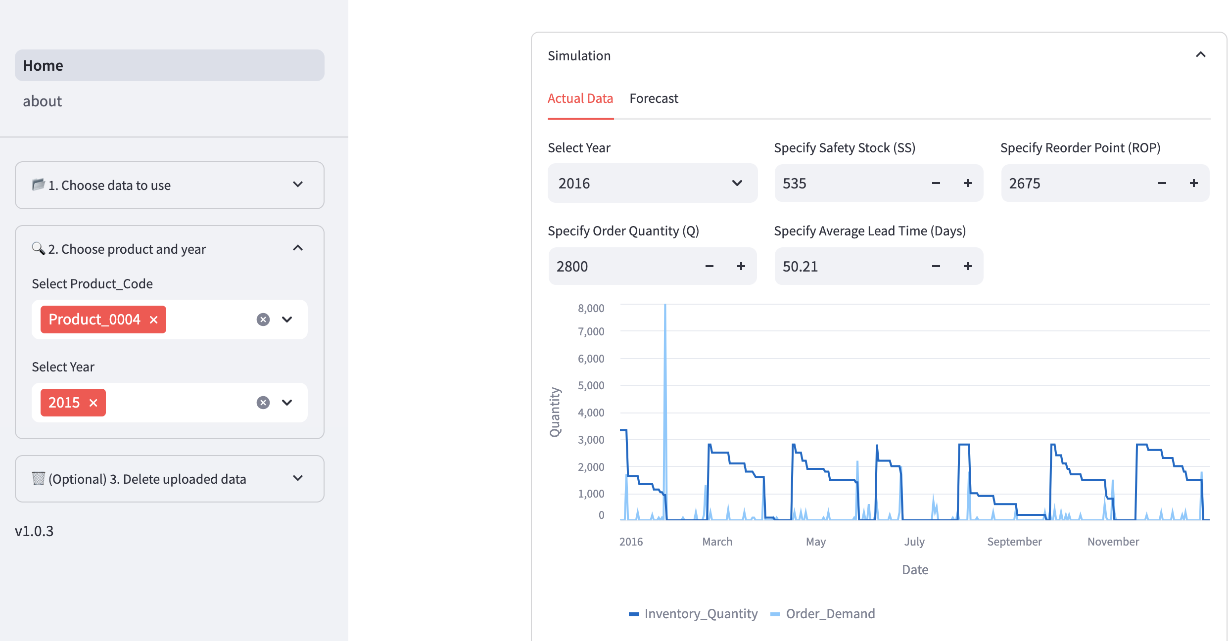
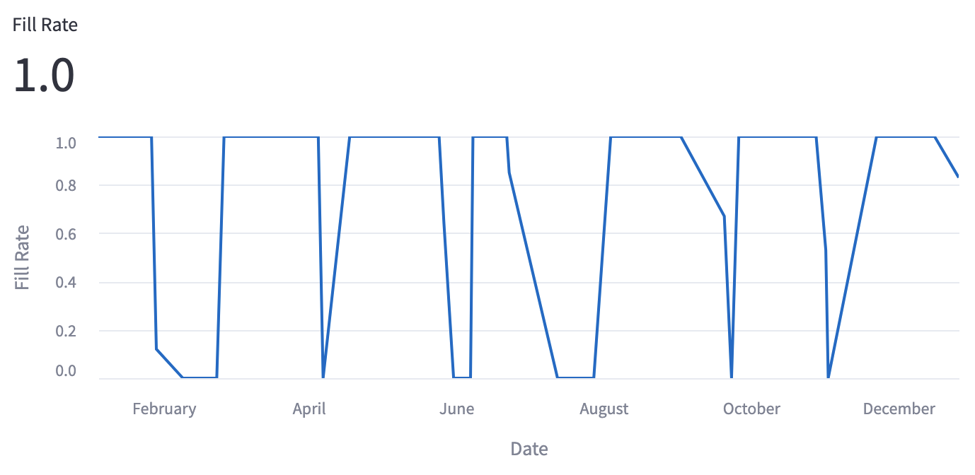
Besides simulating the inventory quantity, I also added the simulation on YTD Fill Rate metric and trend.
Forecasting demand
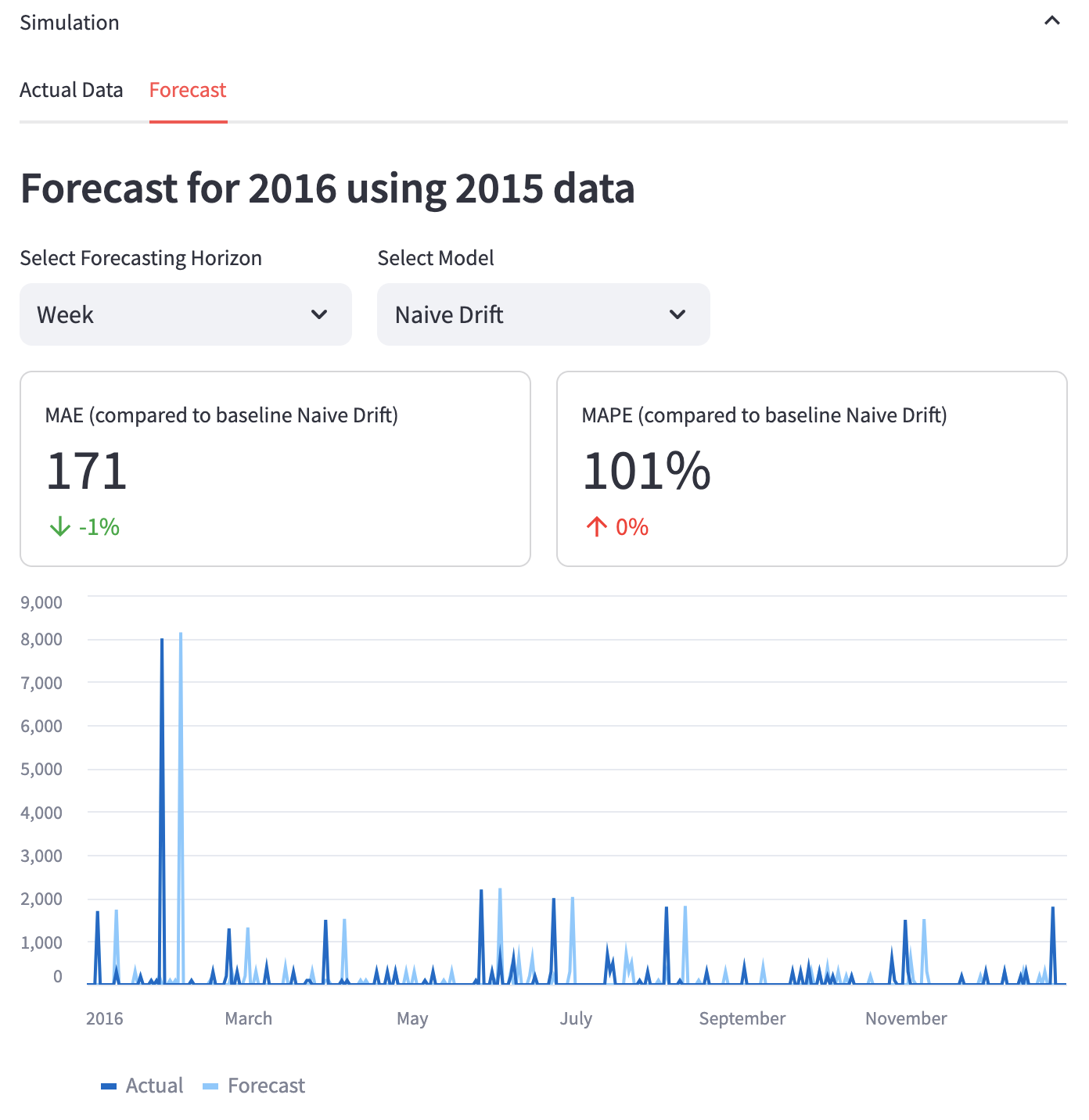
Another main feature of this application is to forecast demand. I designed the application to allow users to validate the models based on past data before forecasting the future. There are 3 forecasting horizons, Day, Week, Month. The model is forecasting in a rolling manner. For example if Week horizon is selected and the week to predict is 2016 Week 2, the model will use 2015 Week 2 - 2016 Week 1 actual data as training data. Subsequently, for 2016 Week 3, the model will use 2015 Week 3 - 2016 Week 2 actual data as training data.
There are 8 forecasting models, Naive Drift, Naive Moving Average, ARIMA, Exponential Smoothing, Theta, Kalman Filter, Linear Regression and Random Forest. Neural networks were excluded as the computational cost outweighed the marginal performance gains for this specific dataset. I used the Darts library for implementing these forecasting models because they provide a consistent way to use various forecasting models, like scikit-learn.
For hyperparameters tuning, the hyperparameters are automatically tuned for each forecast. I used the StatsForecast implementation for ARIMA, Exponential Smoothing and Theta to automatically choose the hyperparameters. For Linear Regression and Random Forest, I specified the parameters grid and used gridsearch method.
Here’s the exact Darts models I have used:
- NaiveDrift
- NaiveMovingAverage
- StatsForecastAutoARIMA
- StatsForecastAutoETS
- StatsForecastAutoTheta
- KalmanForecaster
- LinearRegressionModel
- RandomForest
Mean Absolute Error (MAE) and Mean Absolute Percentage Error (MAPE) were computed for the models’ forecast and compared to the baseline model (Naive Drift). The forecast is plotted over the actual demand.
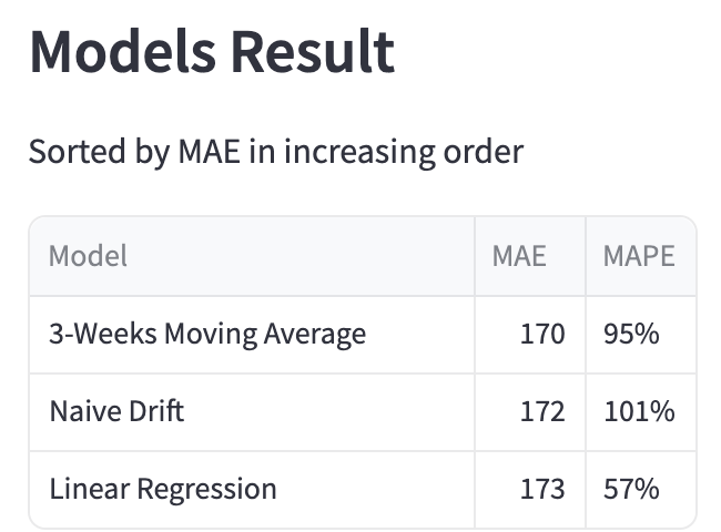
When multiple models are selected, their MAE and MAPE results will be added to a table for comparison.
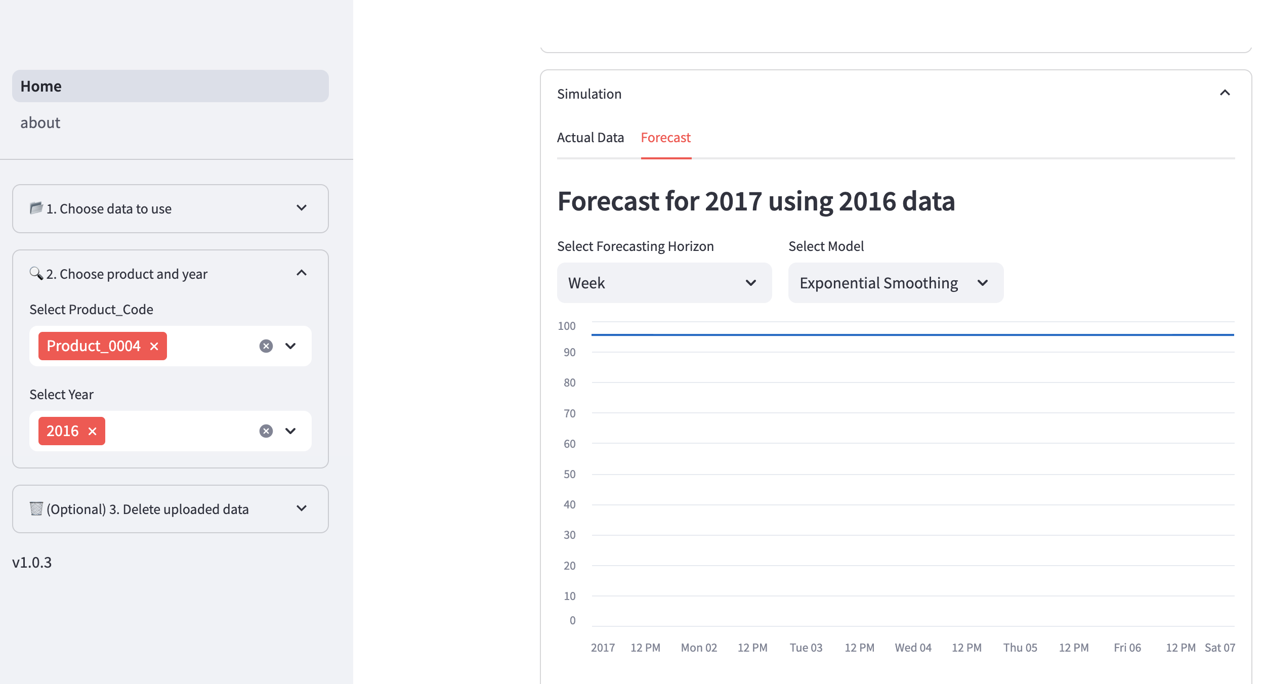
The forecast can be used for inventory simulation similarly as actual demand.
If user select the latest year, the model will forecast 1 day/week/month for the subsequent year.
Uploading custom demand trend and lead time datasets
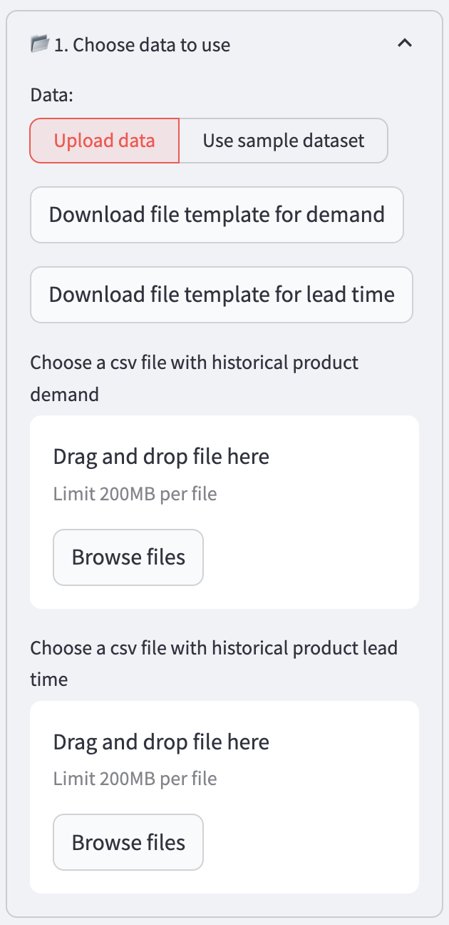
I wanted the app to be more than just a proof-of-concept, so I added the ability for users to upload their own data.
Upon clicking Upload Data, user can download the file templates for demand and lead time, input the values and upload them to this application.
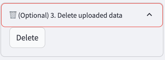
User can delete their uploaded data.
Step 3: Writing Unit Tests and Setting Up Continuous Integration (CI)
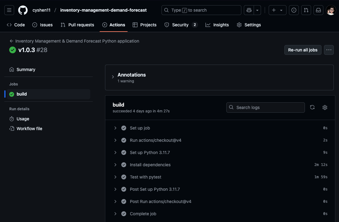
To automatically test the application and ensure future code integrates well, I wrote unit tests using Pytest and Streamlit AppTest.

For CI, I used GitHub Actions and wrote the workflow here. This workflow will run the unit test when the main branch is being pulled or pushed.
Step 4: Deploying the Application and Setting Up Continuous Deployment (CD)
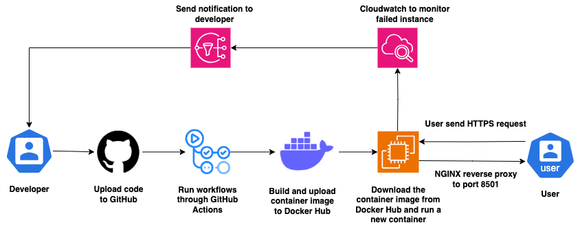
I deployed the application to EC2 using Docker. Before deploying, I prepared this Dockerfile based on this guide Step 2 (Credits to John Davies). GitHub Actions will use this Dockerfile to build a container image of the application.
Next, I launch an EC2 instance with medium size, Ubuntu OS and EBS (28 GB). I tested various instance sizes and found these specs to be the minimum to run my application without crashing. After that, I configured the EC2 instance’s security groups to allow inbound HTTPS, HTTP and SSH traffic. I installed Docker on the EC2.
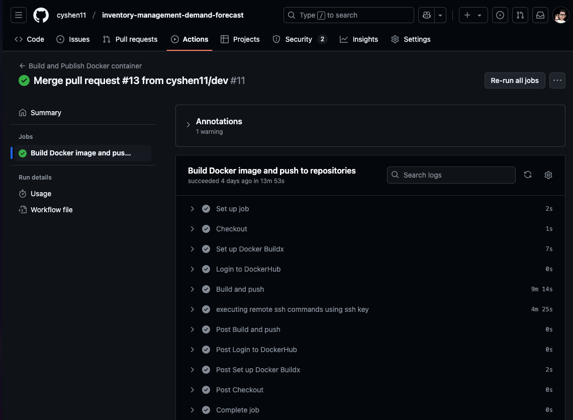
For CD, I used GitHub Actions and wrote the workflow here. This workflow will perform below actions when the main branch is pushed. I also set up Actions secrets for this workflow. Refer to this guide Step 4 for more details on setting up CD pipeline.
- Build the container image
- Upload to Docker Hub
- SSH to EC2
- Stop running container
- Delete existing containers and images
- Download the new container image from Docker Hub
- Run the container image
Step 5: Assigning subdomain to the EC2
After the deployment, I wanted to route my subdomain to the EC2. I allocated an elastic IP address to the EC2 instance to ensure a static IP address. Then, I added the IP address to my subdomain records.
Currently, the Streamlit application is running on port 8501. Hence, I need to setup a webserver to perform reverse proxy from port 443 to 8501 because user will be accessing this application from port 443 (HTTPS) through web browser.
Before setting up the web server, I uploaded my SSL certs to the EC2 as they are part of the prerequisites. If you are using Cloudflare, you can follow this guide on how to get your SSL certs. Next, I installed NGINX on the EC2. I followed this guide on setting up and starting the NGINX. However, this guide’s configuration file is for HTTP (port 80). I modified my configuration file based on this NGINX docmentation to configure for HTTPS server.
Now, when user browse to https://inventory-opt-demand-forecast.vincentcys.com/, they will see the application!

Step 6: Setting up alarm to monitor failed EC2 instances
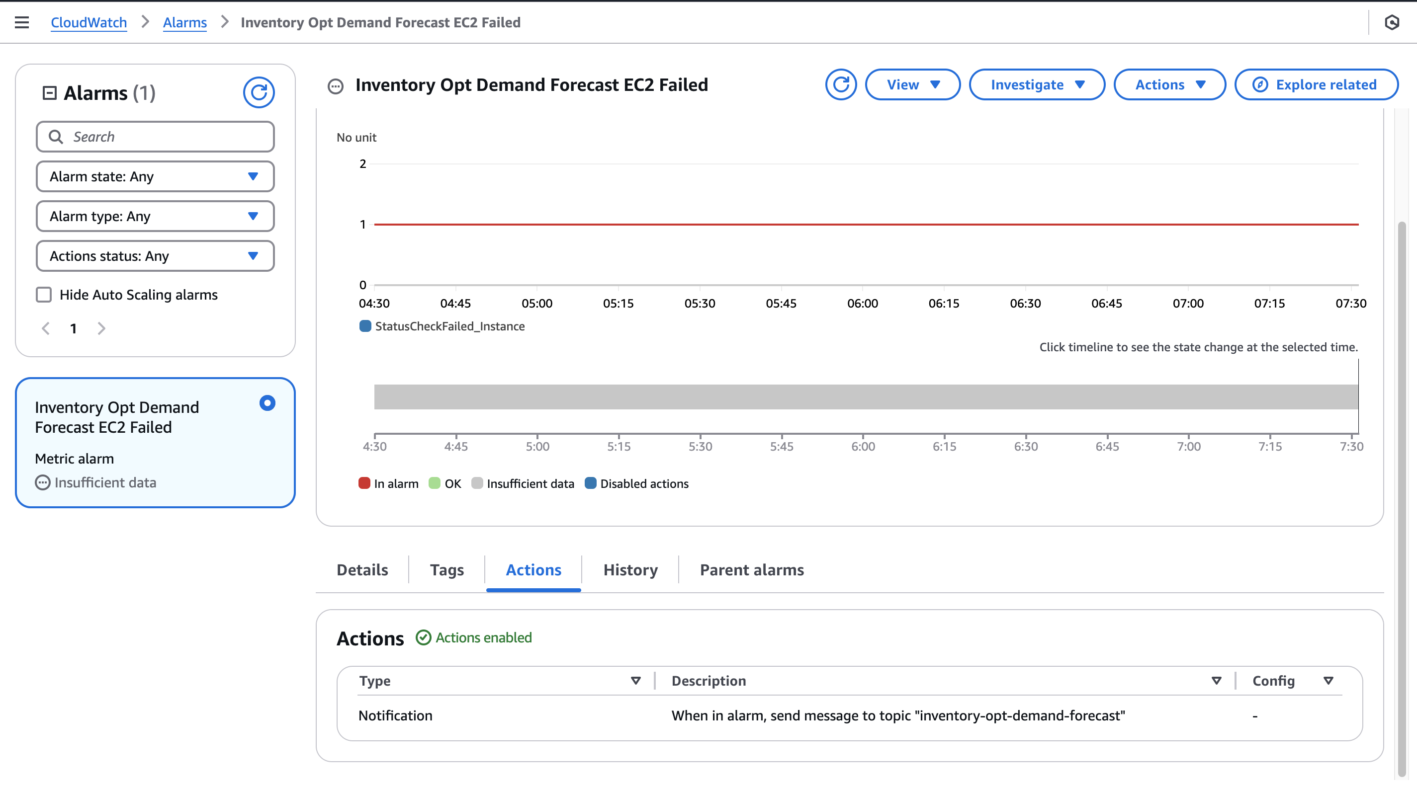
I wanted to be notified if the EC2 instance failed. I setup a Cloudwatch to monitor the EC2 failed instances metric. Next, I setup a SNS with my email address as the subscriber. Upon failure, the Cloudwatch will trigger the SNS to email my email address.
Afterthoughts
DevOps & Reliability: The primary learning outcome of this project was architecting a resilient deployment pipeline. Moving beyond a simple local script, I implemented a robust CI/CD workflow using GitHub Actions and Docker, ensuring that every commit is automatically tested and containerized before reaching the production EC2 instance.
Production Hardening: To simulate a real-world enterprise environment, I placed the application behind an Nginx reverse proxy to handle SSL termination and configure AWS CloudWatch alarms. This ensures high availability and immediate alerting in case of instance failure, bridging the gap between data science and site reliability engineering (SRE).
Future Enhancements
- Improve UI/UX
- Include inventory costing in the simulation
References
Sample Dataset
- Felixzhao, Forecasts for Product Demand
Safety Stock Calculation Formulas
- Edouard Thieuleux, Safety Stock Formula & Calculations
- Safety Stock with Fill Rate Criterion
Deployment
- John Davies, Introduction to deploying an app with simple CI/CD
- Benjamin Franklin. S, Streamlit with Nginx: A Step-by-Step Guide to Setting up Your Data App on a Custom Domain
- Cloudflare, Origin CA certificates
- NGINX, Configuring HTTPS servers